GIS: Terrain Elevated Tinted Hillshade
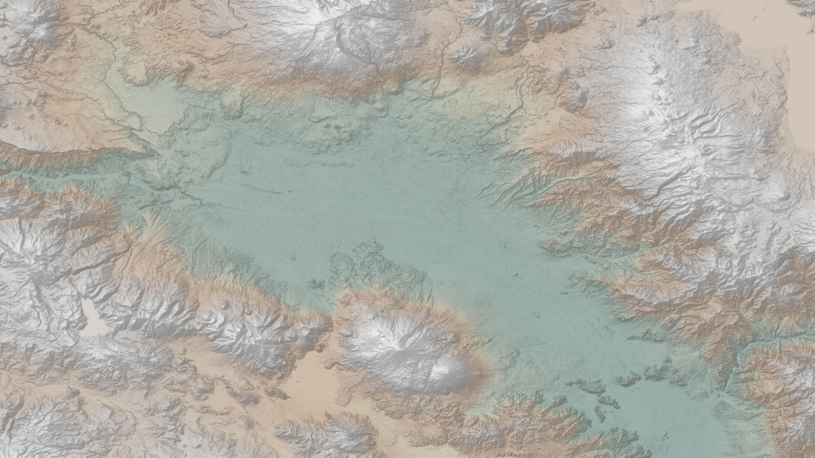
Ever wanted to create hillshaded terrain like the one in this picture? This guide is for you! The area shown here centers over Armenia—a country that should be on your list of places to explore. Look at those mountains! ^_^
Required Data
Prerequisites
- DEM (DSM or DTM) raw files for the region
- GDAL
- QGIS
- GeoServer instance with:
- YSLD plugin
- Image Mosaic plugin
Creating Contoured Hillshade Files
To produce the tinted hillshade, you need elevation data for the area, provided through DEM (Digital Elevation Model) files, which are graphical representations of elevation. DEM files, often in GeoTIFF format, typically contain one band whose values indicate the elevation at each point. Various sources offer elevation data, such as Copernicus DEM, NASA Earthdata, etc.
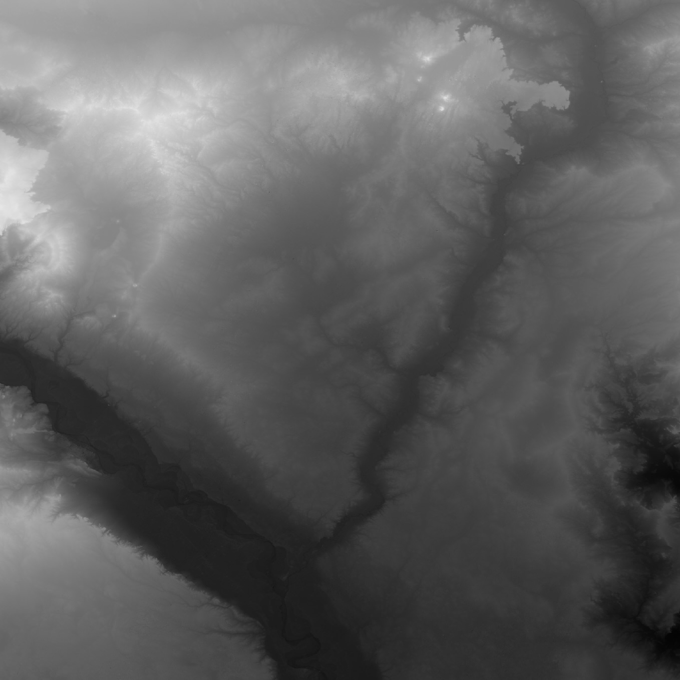
Once you have the DEM data and open it in QGIS, it will appear as a dull gray image like this:
Next, we’ll create contoured hillshades from the raw DEM files.
Script for Generating Hillshaded GeoTIFFs
#!/bin/bash

# Folder containing input files
input_folder="./raw"
hillshade_output_folder="./hillshade"

# Process each file in the input folder
find "$input_folder" -type f -name "*.tif" | while read -r input_file; do
    relative_path="${input_file#$input_folder/}"
    echo $relative_path

    file_directory=$(dirname "$relative_path")
    mkdir -p "$hillshade_output_folder/$file_directory"

    base_name=$(basename "$input_file" .tif)
    output_file="$hillshade_output_folder/$file_directory/${base_name}.tif"

    # Run GDAL command for hillshade
    gdaldem hillshade -s 111120 -z 5 -igor -compute_edges "$input_file" "$output_file"
    echo "Processed $input_file -> $output_file"
done
The main command performing the hillshade transformation is:
gdaldem hillshade -s 111120 -z 5 -igor -compute_edges "$input_file" "$output_file"
- Scale 111120 is for DEM files in EPSG:4326. Omit if using metric coordinates.
- A Z-scale of 5 produces lighter shades.
- The
-igorparameter provides subtle hillshading, ideal for blending with other layers. -compute_edgesis used to avoid grid lines due to missing values in some DEM files.
Applying Colors to DEM Files
Once you have contoured hillshading, apply a color ramp to bring the DEM data to life. My color palette is inspired by The Development and Rationale of Cross-blended Hypsometric Tints, by Patterson & Jenny, with minor adjustments.
To decide on color distribution, I generated a histogram of the overall data. For this, I created a VRT of all raw DEM files and calculated the histogram in QGIS:
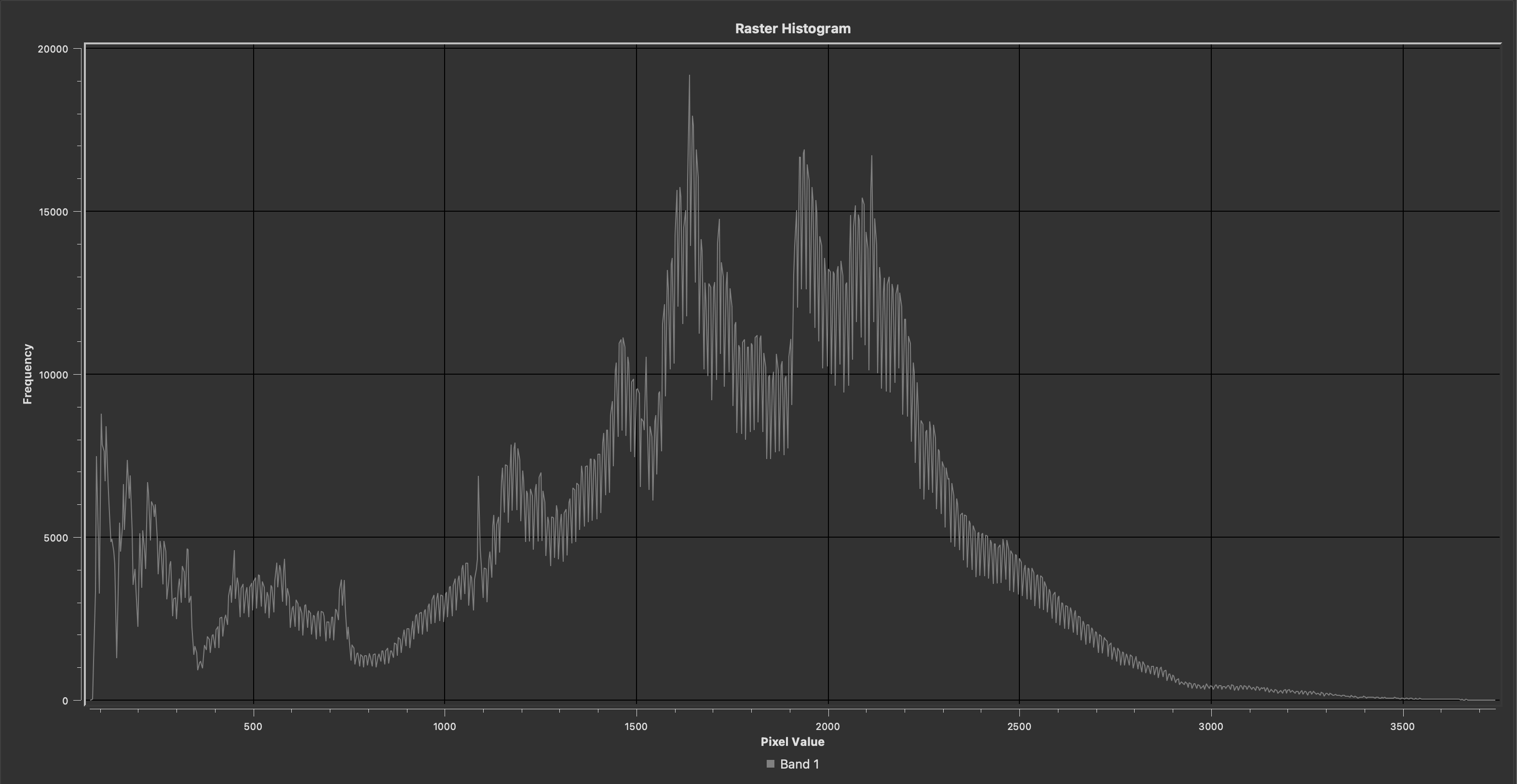
Spikes in the histogram indicate where more color variation is needed to enhance detail. Here’s the final color ramp:
-100 112 137 199 255
70 112 147 141 255
200 120 159 152 255
300 130 165 159 255
700 145 177 171 255
1200 180 192 180 255
1400 212 201 180 255
1600 212 184 163 255
1800 212 193 179 255
2200 212 207 204 255
2400 220 220 220 255
2800 235 235 237 255
3500 245 245 245 255
GeoServer Configuration
Creating GeoServer Stores
- Upload raw and hillshaded GeoTIFF files to your GeoServer filesystem.
- Add indexer.properties files to the raw and hillshade layer folders for Image Mosaic plugin configuration.
indexer.properties
SuggestedFormat=org.geotools.gce.geotiff.GeoTiffFormat
Name=dem-raw-mosaic **OR** dem-hillshade-mosaic
SuggestedSPI=it.geosolutions.imageioimpl.plugins.tiff.TIFFImageReaderSpi
Heterogeneous=false
HeterogeneousCRS=false
PropertyCollectors=CRSExtractorSPI(crs),ResolutionExtractorSPI(resolution)
Schema=*the_geom:Polygon,location:String,crs:String,resolution:String
MosaicCRS=EPSG\:4326 **CHANGE THIS IF NEEDED**
- Create two ImageMosaic stores and publish their layers.
Configuring Styles
Create two styles in GeoServer.
Hillshade Style (YSLD)
name: hillshade
feature-styles:
- x-composite: multiply
  rules:
  - title: raster
    symbolizers:
    - raster:
        opacity: 1.0
        channels:
          gray:
            name: '1'
        channel-selection:
          gray-channel:
            source-channel-name: 1
        color-map:
          type: ramp
          entries:
          - [ "#000000", 0.25, 0, '']
          - [ "#FFFFFF", 1, 255, '']
DEM Style (SLD)
<?xml version="1.0" encoding="ISO-8859-1"?>
<StyledLayerDescriptor version="1.0.0"
  xsi:schemaLocation="http://www.opengis.net/sld StyledLayerDescriptor.xsd"
  xmlns="http://www.opengis.net/sld"
  xmlns:ogc="http://www.opengis.net/ogc"
  xmlns:xlink="http://www.opengis.net/xlink"
  xmlns:xsi="http://www.w3.org/2001/XMLSchema-instance">
  <NamedLayer>
    <Name>Topographic DEM</Name>
    <UserStyle>
      <Title>Topographic DEM</Title>
      <Abstract>A topographic style for DEM data</Abstract>
      <FeatureTypeStyle>
        <Rule>
          <RasterSymbolizer>
            <Opacity>1.0</Opacity>
            <ColorMap type="interval">
              <ColorMapEntry color="#7089C7" quantity="-100" opacity="1.0" />
              <ColorMapEntry color="#70938D" quantity="70" opacity="1.0" />
              <ColorMapEntry color="#789F98" quantity="200" opacity="1.0" />
              <ColorMapEntry color="#82A59F" quantity="300" opacity="1.0" />
              <ColorMapEntry color="#91B1AB" quantity="700" opacity="1.0" />
              <ColorMapEntry color="#B4C0B4" quantity="1200" opacity="1.0" />
              <ColorMapEntry color="#D4C9B4" quantity="1400" opacity="1.0" />
              <ColorMapEntry color="#D4B8A3" quantity="1600" opacity="1.0" />
              <ColorMapEntry color="#D4C1B3" quantity="1800" opacity="1.0" />
              <ColorMapEntry color="#D4CFCC" quantity="2200" opacity="1.0" />
              <ColorMapEntry color="#DCDCDC" quantity="2400" opacity="1.0" />
              <ColorMapEntry color="#EBEBED" quantity="2800" opacity="1.0" />
              <ColorMapEntry color="#F5F5F5" quantity="3500" opacity="1.0" />
            </ColorMap>
          </RasterSymbolizer>
        </Rule>
      </FeatureTypeStyle>
    </UserStyle>
  </NamedLayer>
</StyledLayerDescriptor>
Creating Layer Groups
Create the final layer group with the following layer order:
- dem-raw-mosaic with the dem style.
- dem-hillshade-mosaic with the hillshade style.
Next Steps and Final Thoughts
Once you have the layer group, it is ready to be served! If you found this guide helpful, consider trying it out with other regions or experimenting with different color ramps and hillshade parameters to see the variety of effects you can achieve. Whether you’re mapping for data analysis, design, or just for fun, hillshading opens up a world of possibilities in GIS visualization.